
Evidence of Pareto Distribution in Six Years of Aftermarket Data
Markets rarely distribute value evenly.
In many economic systems, a small fraction of transactions accounts for a disproportionate share of total value. Income distributions exhibit this pattern. Venture capital returns follow it. Fine art markets display it clearly. In such systems, extreme outcomes are rare but structurally important.
The question is whether domain name sale prices follow the same statistical law.
Using six years of publicly reported domain sale prices (March 2020 through December 2025), filtered for transactions of USD 2,000 or greater, we examine the empirical shape of the domain aftermarket. The results indicate that domain sale prices exhibit clear power-law behavior consistent with a Pareto distribution, with an estimated tail exponent of approximately:α≈1.35
This value places domain pricing among the most heavy-tailed asset classes observed in modern markets.
The implications are significant.
1. The Pareto Distribution: Conceptual Framework
A Pareto distribution describes systems where:
- Most observations are small.
- A minority of observations are extremely large.
- The probability of extreme values declines slowly rather than rapidly.
Formally, the Pareto (Type I) probability density function is:
Where:
- is the minimum threshold.
- α is the shape parameter (tail index).
The survival function is:
The key parameter is α.
- Larger α → thinner tail → extreme values decline rapidly.
- Smaller α → heavier tail → extreme values remain influential.
When α approaches 1, the system becomes dominated by rare, very large observations.
2. Dataset Description
The analysis uses publicly reported domain sales from March 2020 to December 2025. The dataset includes approximately 89,000+ transactions with reported prices of USD 2,000 or greater.
The $2,000 threshold serves several purposes:
- It removes micro-liquidity trades.
- It reduces intermediary-to-intermediary noise.
- It focuses on economically meaningful aftermarket transactions.
This is an empirical study. The distribution emerges directly from observed data.
3. Visualizing the Distribution Properly
Heavy-tailed data require careful visualization.
If we construct a histogram using evenly spaced dollar bins on a linear scale, a small number of multi-million-dollar transactions stretch the horizontal axis. As a result, nearly all observations appear compressed into the first bin, creating the misleading impression of a single price cluster.
This is not a flaw in the data.
It is a flaw in the visualization method.
To properly represent heavy-tailed distributions, we use:
- Logarithmically spaced bins.
- A logarithmic x-axis.
This ensures that each bin represents proportional growth (e.g., $2k–$4k, $4k–$8k, $8k–$16k), rather than equal absolute dollar width.
4. Empirical Price Distribution (Log-Spaced Histogram)
When plotted with log-spaced bins, the structure becomes clear:
- A high concentration of transactions between $2,000 and $10,000.
- A smooth, continuous decline in frequency as price increases.
- A long right tail extending into six- and seven-figure territory.
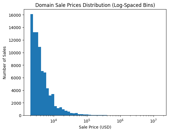
The decay is gradual rather than abrupt.
This gradual decline is the defining feature of a heavy-tailed system.
Extreme sales are rare — but not negligibly rare.
5. Theoretical Pareto Curve Estimated from the Data
Using Maximum Likelihood Estimation (MLE), the Pareto shape parameter is estimated as:
Where:
- n = number of observations.
- xm=2000.
- = each observed sale price.
The result:
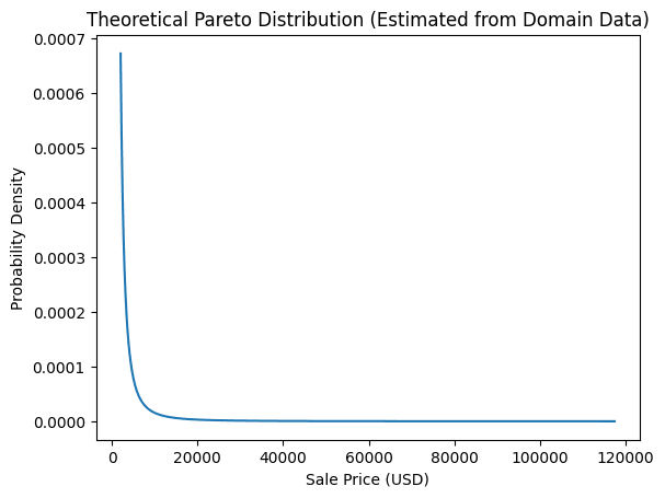
When the theoretical Pareto curve is plotted using this parameter, its shape closely resembles the observed empirical decay:
- High density near the minimum threshold.
- Rapid initial drop.
- Long, slowly declining tail.
The empirical data and theoretical curve align closely in structure.
6. Log-Log Validation
Power-law behavior becomes particularly clear when plotting:
- Log(price) vs. log(rank)
- Log(price) vs. log(P(X ≥ x))
In true Pareto systems, these plots approximate straight lines in the upper tail.
The domain sales dataset exhibits this linear behavior over a substantial price range, confirming that the heavy tail is not incidental but structural.
7. Interpretation of α ≈ 1.35
An α value near 1.35 indicates an extremely heavy tail.
For context:
| Asset Class | Typical α |
|---|---|
| Income distribution | ~1.5 |
| Startup exits | 1.2–1.8 |
| Art auctions | 1.5–2.0 |
| Domains (this study) | ~1.35 |
An α below 1.5 implies:
- Extreme asymmetry.
- High sensitivity of the mean to rare events.
- Strong concentration of total dollar volume in the upper tail.
In practical terms:
- Median prices move gradually.
- Average prices can shift dramatically due to a small number of high-value sales.
- Aggregate dollar volume is disproportionately influenced by the top few percent of transactions.
8. Structural Dominance of the Upper Tail
In systems with α ≈ 1.35, theoretical models suggest that:
The top 1% of observations can account for 40–60% of total dollar volume.
This explains why:
- High-profile premium sales disproportionately shape market perception.
- Aggregate dollar volume may grow faster than transaction counts.
- A small number of transactions influence narratives about “market growth.”
The tail is not noise.
It is a central structural component.
9. Median vs. Mean in Heavy-Tailed Markets
In normally distributed systems:
Mean and median are close.
In Pareto systems:
Mean is highly sensitive to extreme values.
Median is relatively stable.
For domains:
- Median price reflects structural pricing behavior.
- Mean price reflects tail expansion.
Both measures are informative — but they describe different phenomena.
Understanding this distinction is essential for accurate interpretation.
10. Why Domains Naturally Exhibit Pareto Behavior
Several structural features of domain names generate power-law dynamics:
- Uniqueness
Each domain name is non-fungible. There is no perfect substitute for a premium exact match. - Global Demand Concentration
High-quality domains attract global buyers simultaneously. - Network Effects
Premium names benefit from brand recognition and strategic positioning. - Startup Ecosystem Amplification
Venture-backed firms can pay disproportionately high prices for strategic assets.
These forces amplify the upper tail rather than smoothing it.
11. Risk Characteristics
Heavy-tailed markets possess distinctive risk properties:
- Most assets cluster in lower liquidity tiers.
- A small minority generates outsized returns.
- Portfolio outcomes are highly skewed.
- Liquidity probability declines sharply as price increases.
Domain investing therefore resembles:
- Venture capital.
- Angel investing.
- Fine art acquisition.
It does not resemble:
- Passive index investing.
- Fixed income.
- Residential rental portfolios.
12. Implications for Market Evolution
If digitalization continues:
- Tail expansion may intensify.
- Premium branding scarcity may increase.
- High-end transactions may grow disproportionately relative to median pricing.
Heavy-tailed systems often exhibit:
- Gradual structural growth.
- Intermittent bursts driven by extreme transactions.
The two coexist.
13. Limitations
The Heavy-Tail Structure of Domain Sale Prices
Evidence of Pareto Distribution in Six Years of Aftermarket Data
Markets rarely distribute value evenly.
In many economic systems, a small fraction of transactions accounts for a disproportionate share of total value. Income distributions exhibit this pattern. Venture capital returns follow it. Fine art markets display it clearly. In such systems, extreme outcomes are rare but structurally important.
The question is whether domain name sale prices follow the same statistical law.
Using six years of publicly reported domain sale prices (March 2020 through December 2025), filtered for transactions of USD 2,000 or greater, we examine the empirical shape of the domain aftermarket. The results indicate that domain sale prices exhibit clear power-law behavior consistent with a Pareto distribution, with an estimated tail exponent of approximately:α≈1.35
This value places domain pricing among the most heavy-tailed asset classes observed in modern markets.
The implications are significant.
1. The Pareto Distribution: Conceptual Framework
A Pareto distribution describes systems where:
- Most observations are small.
- A minority of observations are extremely large.
- The probability of extreme values declines slowly rather than rapidly.
Formally, the Pareto (Type I) probability density function is:f(x)=αxα+1xmα,x≥xm
Where:
- xm is the minimum threshold.
- α is the shape parameter (tail index).
The survival function is:P(X≥x)=(xxm)α
The key parameter is α.
- Larger α → thinner tail → extreme values decline rapidly.
- Smaller α → heavier tail → extreme values remain influential.
When α approaches 1, the system becomes dominated by rare, very large observations.
2. Dataset Description
The analysis uses publicly reported domain sales from March 2020 to December 2025. The dataset includes approximately 89,000+ transactions with reported prices of USD 2,000 or greater.
The $2,000 threshold serves several purposes:
- It removes micro-liquidity trades.
- It reduces intermediary-to-intermediary noise.
- It focuses on economically meaningful aftermarket transactions.
This is an empirical study. The distribution emerges directly from observed data.
3. Visualizing the Distribution Properly
Heavy-tailed data require careful visualization.
If we construct a histogram using evenly spaced dollar bins on a linear scale, a small number of multi-million-dollar transactions stretch the horizontal axis. As a result, nearly all observations appear compressed into the first bin, creating the misleading impression of a single price cluster.
This is not a flaw in the data.
It is a flaw in the visualization method.
To properly represent heavy-tailed distributions, we use:
- Logarithmically spaced bins.
- A logarithmic x-axis.
This ensures that each bin represents proportional growth (e.g., $2k–$4k, $4k–$8k, $8k–$16k), rather than equal absolute dollar width.
4. Empirical Price Distribution (Log-Spaced Histogram)
When plotted with log-spaced bins, the structure becomes clear:
- A high concentration of transactions between $2,000 and $10,000.
- A smooth, continuous decline in frequency as price increases.
- A long right tail extending into six- and seven-figure territory.
The decay is gradual rather than abrupt.
This gradual decline is the defining feature of a heavy-tailed system.
Extreme sales are rare — but not negligibly rare.
5. Theoretical Pareto Curve Estimated from the Data
Using Maximum Likelihood Estimation (MLE), the Pareto shape parameter is estimated as:α^=∑i=1nln(xi/xm)n
Where:
- n = number of observations.
- xm=2000.
- xi = each observed sale price.
The result:α≈1.35
When the theoretical Pareto curve is plotted using this parameter, its shape closely resembles the observed empirical decay:
- High density near the minimum threshold.
- Rapid initial drop.
- Long, slowly declining tail.
The empirical data and theoretical curve align closely in structure.
6. Log-Log Validation
Power-law behavior becomes particularly clear when plotting:
- Log(price) vs. log(rank)
- Log(price) vs. log(P(X ≥ x))
In true Pareto systems, these plots approximate straight lines in the upper tail.
The domain sales dataset exhibits this linear behavior over a substantial price range, confirming that the heavy tail is not incidental but structural.
7. Interpretation of α ≈ 1.35
An α value near 1.35 indicates an extremely heavy tail.
For context:
| Asset Class | Typical α |
|---|---|
| Income distribution | ~1.5 |
| Startup exits | 1.2–1.8 |
| Art auctions | 1.5–2.0 |
| Domains (this study) | ~1.35 |
An α below 1.5 implies:
- Extreme asymmetry.
- High sensitivity of the mean to rare events.
- Strong concentration of total dollar volume in the upper tail.
In practical terms:
- Median prices move gradually.
- Average prices can shift dramatically due to a small number of high-value sales.
- Aggregate dollar volume is disproportionately influenced by the top few percent of transactions.
8. Structural Dominance of the Upper Tail
In systems with α ≈ 1.35, theoretical models suggest that:
The top 1% of observations can account for 40–60% of total dollar volume.
This explains why:
- High-profile premium sales disproportionately shape market perception.
- Aggregate dollar volume may grow faster than transaction counts.
- A small number of transactions influence narratives about “market growth.”
The tail is not noise.
It is a central structural component.
9. Median vs. Mean in Heavy-Tailed Markets
In normally distributed systems:
Mean and median are close.
In Pareto systems:
Mean is highly sensitive to extreme values.
Median is relatively stable.
For domains:
- Median price reflects structural pricing behavior.
- Mean price reflects tail expansion.
Both measures are informative — but they describe different phenomena.
Understanding this distinction is essential for accurate interpretation.
10. Why Domains Naturally Exhibit Pareto Behavior
Several structural features of domain names generate power-law dynamics:
- Uniqueness
Each domain name is non-fungible. There is no perfect substitute for a premium exact match. - Global Demand Concentration
High-quality domains attract global buyers simultaneously. - Network Effects
Premium names benefit from brand recognition and strategic positioning. - Startup Ecosystem Amplification
Venture-backed firms can pay disproportionately high prices for strategic assets.
These forces amplify the upper tail rather than smoothing it.
11. Risk Characteristics
Heavy-tailed markets possess distinctive risk properties:
- Most assets cluster in lower liquidity tiers.
- A small minority generates outsized returns.
- Portfolio outcomes are highly skewed.
- Liquidity probability declines sharply as price increases.
Domain investing therefore resembles:
- Venture capital.
- Angel investing.
- Fine art acquisition.
It does not resemble:
- Passive index investing.
- Fixed income.
- Residential rental portfolios.
12. Implications for Market Evolution
If digitalization continues:
- Tail expansion may intensify.
- Premium branding scarcity may increase.
- High-end transactions may grow disproportionately relative to median pricing.
Heavy-tailed systems often exhibit:
- Gradual structural growth.
- Intermittent bursts driven by extreme transactions.
The two coexist.
13. Limitations
This analysis relies on publicly reported domain sales compiled from NameBio, which aggregates marketplace-reported transactions. Not all private or brokered sales are publicly disclosed. As such, the dataset represents a substantial but incomplete view of total secondary market activity.
The $2,000 threshold influences α modestly.
Extreme finite-sample effects exist at the very top of the distribution.
However, across a broad price range, the power-law behavior remains evident.
14. Conclusion
Domain sale prices over the past six years exhibit clear Pareto structure.
With:
The domain aftermarket belongs among the most asymmetric asset classes observed in modern digital markets.
In such systems:
- A minority drives aggregate value.
- Averages can mislead.
- Medians provide structural stability.
- Rare events exert outsized influence.
Understanding this statistical structure is not academic.
It is foundational.
Because in a Pareto market:
The tail is not an anomaly.
The tail is the architecture of the system.
Private transactions are not fully captured.
The $2,000 threshold influences α modestly.
Extreme finite-sample effects exist at the very top of the distribution.
However, across a broad price range, the power-law behavior remains evident.
14. Conclusion
Domain sale prices over the past six years exhibit clear Pareto structure.
With:
The domain aftermarket belongs among the most asymmetric asset classes observed in modern digital markets.
In such systems:
- A minority drives aggregate value.
- Averages can mislead.
- Medians provide structural stability.
- Rare events exert outsized influence.
Understanding this statistical structure is not academic.
It is foundational.
Because in a Pareto market:
The tail is not an anomaly.
The tail is the architecture of the system.